Selection of the Loss Functions for Logistic Regression

When training a machine learning model, choosing the right loss function is critical to ensuring effective learning. In linear regression, Mean Squared Error (MSE) is commonly used, but for logistic regression, it becomes problematic.

In this post, we’ll explore why MSE is not suitable for logistic regression and why cross-entropy loss (log-loss) is the better choice.

When to Use Logistic Regression:

• Binary Classification: When the dependent variable has two categories.
  • Example: Predicting whether an email is “spam” or “not spam.”
• Probability Estimation: When you need to estimate the probability of an event occurring.
  • Example: Estimating the likelihood of a customer purchasing a product based on their browsing behavior.
• Understanding Relationships: When you aim to understand the impact of independent variables on the likelihood of a particular outcome.
  • Example: Assessing how factors like age, income, and education level influence the probability of loan default.

Understanding Logistic Regression

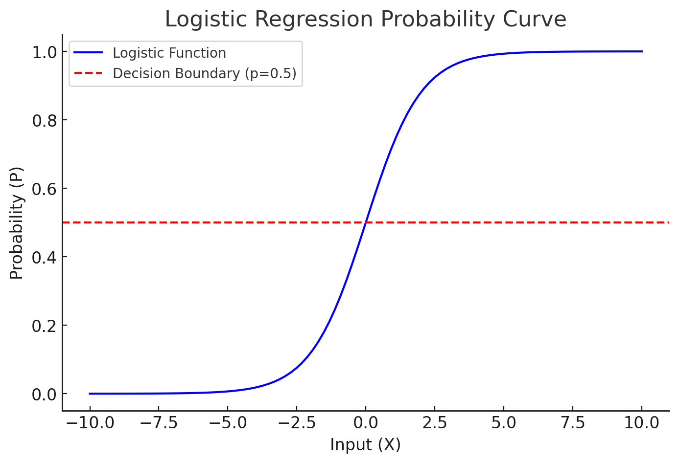
Logistic regression is a classification algorithm used to predict binary outcomes (0 or 1). Instead of modeling a continuous output like linear regression, it models probabilities using the sigmoid activation function:

where:

• \( \hat{y} \) is the predicted probability.
• \( z = Xw + b \) is the linear combination of inputs and weights.
• \( \sigma(z) \) (sigmoid function) ensures the output is in the range \([0,1]\).

Since logistic regression is used for classification, our goal is to maximize the likelihood of correctly predicting class labels. In order to learn the logistric regression, the immediate step is to decide which loss function to choose to represent the difference between groundth \( y \) and predicted \( \hat{y} \) value. The common choose of loss functions are Mean Square Error (MSE) and Cross Entropy.

Why Not Use MSE for Logistic Regression?

We will start with MSE. MSE is defined as:

However, using MSE in logistic regression causes three major problems:

1. MSE Leads to a Non-Convex Loss Function

• The sigmoid function introduces non-linearity, and when combined with MSE, the loss function becomes non-convex.
• Gradient descent struggles to converge efficiently because it can get stuck in local minima.
• Cross-entropy loss is convex, ensuring faster and more stable convergence.

2. MSE Treats Probabilities as Continuous Values

• Logistic regression models probabilities, but MSE assumes continuous errors, which is not optimal for classification.
• Example: If the actual label is 1, and the model predicts 0.9, MSE gives a small loss, but in classification, we need a sharper distinction.

3. MSE Leads to Small Gradients (Slow Learning)

The gradient of MSE with respect to weights:

When \(\hat{y}\) is close to 0 or 1, the term \(\hat{y} (1 - \hat{y})\) becomes very small, leading to vanishing gradients.

• This slows down learning and makes convergence inefficient.

Why Cross-Entropy Loss is Better

Instead of MSE, logistic regression uses cross-entropy loss:

Key Benefits of Cross-Entropy Loss:

✔ Convex loss function → Ensures faster & more stable convergence.
✔ Better probability modeling → Matches the Bernoulli distribution.
✔ Prevents small gradient issues → Ensures meaningful weight updates.

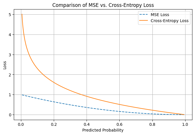
Visualization: Comparing MSE vs. Cross-Entropy Loss

To better understand the difference, let’s visualize how MSE vs. Cross-Entropy Loss behave for classification.

Optimizer

Now that we decided to use the Cross Entropy for loss function. To use the loss function to guide the changes of the weights and bias, we need to take the gradient of the loss function.

Learn with Code

"""
------ Psudo Code------ 
# Train logistic regression model
model = LogisticRegression()
model.fit(X_train, y_train)
# Predict probabilities for test set
y_probs = model.predict_proba(X_test)[:, 1]  # Probability for class 1 (relevant)
# Rank items based on predicted probabilities
ranking = np.argsort(-y_probs)  # Negative sign for descending order
------ Basic function ------


"""

import numpy as np
"""
Basic function
"""

def pred (X,w):
  # X: Input features, w: Weights
  # y hat = sig (1/ 1+e^-z), z = wx +b
  z = np.matmul(X,w)
  y_hat = 1/(1+np.exp(-z))
  return y_hat

def loss(X,Y,w):
  # Compute the binary cross-entropy loss
  # Loss is not directly used in the train,g but its gradient is used to update the weights
  y_pred  = pred(X, w)
  sum = - Y * np.log(y_pred) + (1-Y) * np.log(1-y_pred)
  return - np.mean (sum)


def gradient (X,Y,w):
  # Derivative of Loss to w and b
  #	The gradient of the loss function tells us the direction and magnitude in which the model’s parameters should be adjusted to minimize the loss.
  y_pred  = pred(X, w)
  g =  - np.matmul(  X.T, (y_pred- Y) ) / X.shape[0]
  return g

"""
Phase of training and testing
"""
def train(X,Y, iter= 10000, learning_rate = 0.002):
   w = np.zeros((X.shape[1],1)) # w0 intialization at Zero
   for i in range(iter):
    w = w - learning_rate * gradient(X,Y,w)
    y_pred = pred(X,w)
    if i % 1000 == 0:
      print (f"iteration {i}, loss = { loss(X,Y,w)}" )

   return w

def test(X,Y, w):
  y_pred = pred(X,w)
  y_pred_labels = (y_pred > 0.5).astype(int)
  accuracy = np.mean(y_pred_labels == Y)
  return accuracy

🤖 Disclaimer: This post was generated with the help of AI but reviewed, refined, and enhanced by Dr. Rebecca Li, blending AI efficiency with human expertise for a balanced perspective.